In a word, no. Â But the relationship between consistency and speed is a little subtle. Â To look at this question let’s take the distance results from major international competitions (OWG, WSC or World Cups) and restrict ourselves to those times when an athlete did at least ten races in a particular season. Â Then for each season we’ll calculate a how variable their results were and also the average of their best five races.I’m going to use FIS points as my measure, but the adjusted version that I’ve created myself to account for differences between mass start and interval start races and changes in the F-factors over time. Â The “standard” way to measure variability is the standard deviation (SD). Â This can be a bit sensitive to single outliers, though, and we’re only requiring a minimum of ten races so we’ll also consider the more robust median absolute deviation (MAD), just for kicks.
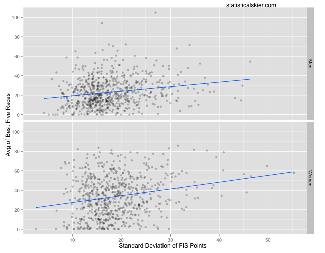
Here’s a look at the results using SD:
And here’s the same plot using MAD:
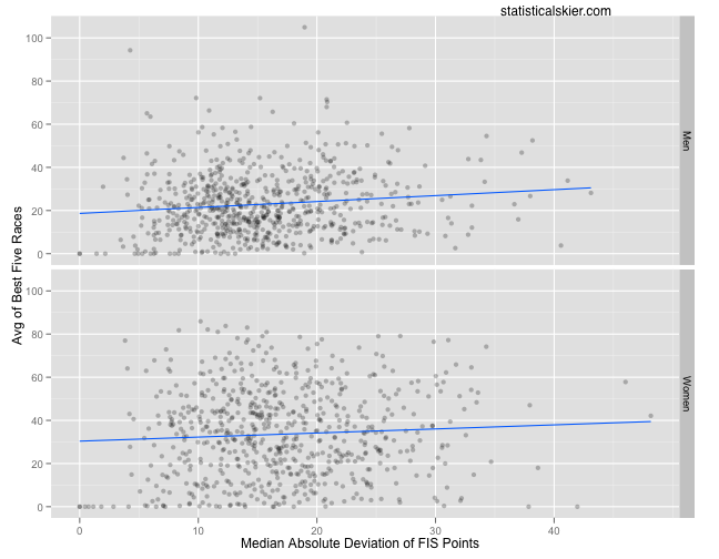
 Here’s where we need to start being careful, and where I start doling out statistics lessons. Â Our question is whether consistent skiers (low variability) tend to ski faster (low average of best five FIS points). Â Technically, then, we’re looking to see whether the slopes of the blue lines are positive.
And they are. Â Just look at ’em! Â Case closed, right?
Not really. Â First of all we can see that there’s clearly a difference between using SD and MAD. Â Namely, this relationship seems less pronounced using the more robust MAD. Â I’m inclined to prefer MAD in this case. Â The SD might not really capture the “typical” level of variability since it can easily be inflated by a single very bad race.
Even so, the lines are sloping upward even in the MAD version of the plots. Â Now, you might be thinking that I’m going to pull some sort of “this isn’t actually statistically significant” trick out of my hat. Â But I’m not:
| Estimate | Std. Error | t value | p value | |
|---|---|---|---|---|
| Intercept | 14.5583 | 1.9744 | 7.37 | 0.0000 |
| SD of FIS Points | 0.4716 | 0.1051 | 4.49 | 0.0000 |
| Gender (Women) | 5.8085 | 2.8971 | 2.00 | 0.0452 |
| SD:Gender | 0.2261 | 0.1493 | 1.51 | 0.1302 |
| Estimate | Std. Error | t value | p value | |
|---|---|---|---|---|
| Intercept | 18.6618 | 1.7301 | 10.79 | 0.0000 |
| MAD of FIS Points | 0.2749 | 0.1033 | 2.66 | 0.0079 |
| Gender (Women) | 11.7077 | 2.5020 | 4.68 | 0.0000 |
| MAD:Gender | -0.0862 | 0.1424 | -0.61 | 0.5452 |
If you aren’t a stat-head, these might be more intimidating than some pretty graphs. Â It’s just a really simple regression model, one each for the SD and MAD versions. Â We only need to focus on the second and fourth rows of each table for now.
The second row gives us the estimated slope for men, and we get the estimated slope for women by adding this to the estimate in the fourth row. Â So for the SD model, the slope for the men is about 0.4716 and for the women it’s about 0.6977. Â And the p-values suggest that this relationship is quite statistically significant! Â The results for the MAD version suggest a smaller slope, but it still looks statistically significant. Â (The larger p-values in the fourth row indicates a lack of statistical significance between the slopes for the men and women.)
There’s an enormous amount of variation around this relationship we’ve found, indicated by how spread out the points are around the blue lines in the graphs above. Â The relationship exists, “on average”, but accounts for very little of the variability in the data (the R-Squared values were 0.12 and 0.08 respectively, if you care for that sort of thing).
This suggests that more consistent skiers are, on average, faster, but only slightly and if we listed the factors influencing how fast skiers go in order of importance, consistency would likely be way down near the bottom.
This is a great example of how statistics can provide information, but not necessarily an answer. Â Sadly, when people ask statisticians for help, they usually want an answer.

Post a Comment